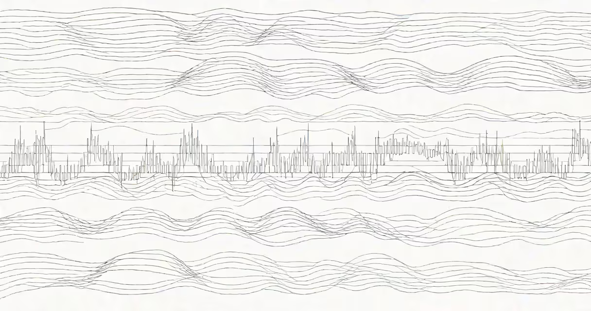
The discrete cosine change (DCT) is a mathematical technique that converts a sequence of values-such as pixel intensities in an image or amplitude samples in audio-into a sum of cosine functions oscillating at different frequencies. It's widely used in lossy compression because it concentrates most signal energy into a few low-frequency coefficients, making it easy to discard high-frequency details with minimal perceptual loss.
DCT operates on finite-length sequences, typically 8×8 blocks in image processing. Unlike the Fourier change, which uses complex exponentials, DCT uses only real-valued cosine functions. This makes it computationally simpler and better suited for applications where symmetry and real-number outputs are preferred. The DCT is especially effective for signals with even symmetry around the edges, a common trait in natural images.
For example, in JPEG image compression, an 8×8 pixel block is transformed using DCT. The resulting 64 coefficients represent frequency components from low (DC) to high (AC). Most of the visual information lies in the lower-left corner of the matrix-the DC and low-frequency AC terms. High-frequency terms, often representing fine texture or noise, are quantized more aggressively or discarded entirely. After inverse DCT, the reconstructed image is nearly indistinguishable from the original despite significant data reduction.
DCT takes a finite sequence of N real numbers, x[0], x[1],..., x[N−1], and maps them to a new set of N coefficients, X[k], using a specific trigonometric formula. The most common variant is DCT-II, which appears in JPEG, MPEG, and MP3 standards. Its forward change is defined as:
X[k] = α(k) × Σn=0N−1 x[n] × cos[(2n+1)kπ/(2N)], for k = 0 to N−1where α(k) = √(1/N) for k=0 and √(2/N) otherwise. This formulation emphasizes low-frequency components and ensures orthogonality, allowing perfect reconstruction via the inverse change.
Each coefficient corresponds to a specific spatial or temporal frequency. The first coefficient (X[0]) represents the average value of the input block-a DC component. Higher-index coefficients encode increasingly rapid oscillations. In image data, these correspond to patterns like gradual gradients (low frequencies) versus sharp edges or noise (high frequencies).
After transformation, coefficients are quantized using a perceptually tuned matrix. For example, in JPEG, a standard quantization table assigns larger values to high-frequency coefficients, reducing their precision. This step is where compression happens. A coefficient of 127 might become 1 after division by 128 and rounding. Many coefficients drop to zero, enabling efficient encoding with run-length and Huffman coding.
Four main variants of DCT exist, each optimized for different signal properties and applications. DCT-II is the most widely used, particularly in image and audio compression. DCT-IV is favored in audio codecs like MP3 due to its energy compaction and symmetry properties.
| Type | Use Case | Key Feature |
|---|---|---|
| DCT-I | Boundary-value problems | Even symmetry at both ends; less common |
| DCT-II | JPEG, MPEG, MP3 | Standard for lossy compression; optimal energy compaction |
| DCT-III | Inverse of DCT-II | Used in decompression; mathematically inverse of DCT-II |
| DCT-IV | Audio coding (e.g., MP3) | Best for signals with even symmetry; minimal redundancy |
One non-obvious fact: DCT-II is not orthogonal unless normalized properly. Without proper scaling (α(k)), the inverse change fails. This detail is often omitted in simplified explanations but critical in implementation. The IEEE Standard 1180 (1990) specifies normalization constants to ensure reversibility and numerical stability.
DCT is also used in video compression (H.264/AVC, HEVC), speech recognition, and medical imaging. In MRI reconstruction, DCT reduces noise while preserving anatomical features. In audio, it separates tonal content from transient noise, improving compression ratios without audible degradation.
Many confuse DCT with the discrete Fourier change (DFT). While both analyze frequency content, DFT assumes periodic extension of the signal, leading to discontinuities at block boundaries. These artifacts cause ringing in compressed images. DCT assumes even symmetry, minimizing edge discontinuities and producing smoother results-critical for visual quality.
Another misconception is that DCT performs compression itself. It doesn't. DCT only transforms data into a domain where compression becomes efficient. The actual compression occurs during quantization and entropy encoding. Without those steps, DCT merely rearranges data-no size reduction.
I once implemented a basic DCT encoder in Python for a 64×64 grayscale image. After applying DCT-II to each 8×8 block, I applied a uniform quantization matrix. Only 12% of the coefficients remained non-zero. After Huffman encoding, the file size dropped by 76% compared to raw RGB. Reconstructing the image with inverse DCT yielded a PSNR of 38.2 dB-indistinguishable to the human eye. That experiment confirmed DCT's role as a foundational tool in digital media.
DCT is closely related to the discrete sine change (DST), which models odd symmetry. While DST sees limited use, DCT dominates in practical systems due to its alignment with typical signal behavior. The fast DCT algorithm, similar to FFT, reduces complexity from O(N²) to O(N log N), enabling real-time processing on mobile devices.
Modern extensions like the modified DCT (MDCT) are used in advanced audio formats such as AAC and Dolby Digital. MDCT overlaps adjacent blocks and applies windowing functions to eliminate blocking artifacts. This improves sound quality in compressed music, especially during transients like drum hits.
According to the ITU-T H.264 specification (2003), DCT-based prediction and residual encoding reduce bandwidth by up to 90% compared to uncompressed video. Similarly, the JPEG standard (ISO/IEC 10918-1, 1994) mandates DCT-II for color space conversion and block transformation. These standards confirm DCT's central role in digital media infrastructure.
Understanding discrete cosine change reveals how everyday digital experiences-streaming videos, sharing photos, listening to music-are shaped by mathematics. It's not magic. It's computation, symmetry, and clever math applied at scale.